Introduction
I was recently enrolled in an online course called “Full Stack Deep Learning in AWS”, organized by AICamp. It was a 4-week 8-session course that started on Jun 15, 2020 (batch #6). The overarching theme of the course was about production-ready end-to-end machine learning in Amazon Web Services (AWS), from uploading datasets, training/testing a model, all the way to deploying the model to the external world, all using AWS ecosystem (e.g. S3, SageMaker, Lambda, API Gateway). A good amount of deep learning theory was covered for deep learning for image classification (CNN/ResNet) and time series forecasting (RNN/LSTM/DeepAR).
To demonstrate our understanding of the contents, we have to work on a capstone project in order to complete the course. For my capstone project, I decided to work on a flower image classification problem using data from Kaggle. The deep learning model training was done using the Image Classification (ResNet) algorithm in AWS SageMaker and the best trained model was exposed externally as a REST API.
Problem Statement and Data Analysis
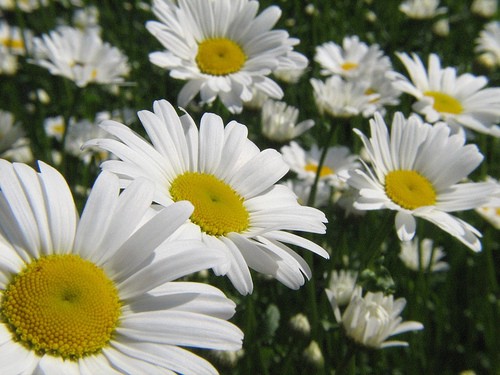
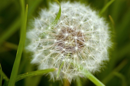
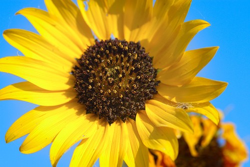
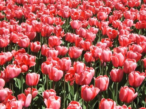
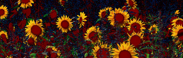
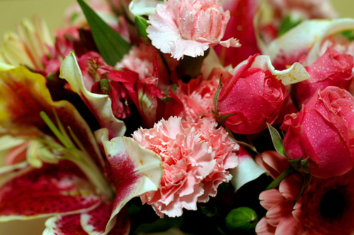
This capstone project is about training an image classifier using deep learning that can identify 5 different types of flowers:

The flower image dataset used for training was obtained from Kaggle: https://www.kaggle.com/alxmamaev/flowers-recognition/data. According to the author, the images were collected from Flickr, Google images and Yandex images.
The flowers in the images vary a lot within each category. There are close up shots, far shots, images taken from different angles, and flowers of different colors within the same class. This captures a wide variety of real-world situations which helps to train a more robust model. This is something that Convolution Neural Networks (CNN) are able to handle.
Since the training data are images, the features are basically just the RGB image pixels.
Feature Engineering
Distribution
The flowers dataset is not balanced and are distributed as such:
- daisy: 769
- dandelion: 1055 (max)
- rose: 784
- sunflower: 734 (min)
- tulip: 984
for a total of 4242 images.
Resolution
All the images are 3-channel RGB colored images, and they vary in resolution, ranging from around 240×240 to 320×320. They also vary in width-height proportions.
Training Input
AWS SageMaker requires lst files that lists train/validation images in the following format, one image per line:
[image_id] [class_id] [relative_path_to_image]
For example:
0 0 daisy/8071646795_2fdc89ab7a_n.jpg
1 0 daisy/34326606950_41ff8997d7_n.jpg
2 1 dandelion/2503875867_2075a9225d_m.jpg
3 1 dandelion/12094442595_297494dba4_m.jpg
4 3 sunflower/6050020905_881295ac72_n.jpg
5 2 rose/5088766459_f81f50e57d_n.jpg
7 4 tulip/16862422576_5226e8d1d0.jpg
8 1 dandelion/2330339852_fbbdeb7306_n.jpg
9 1 dandelion/854593001_c57939125f_n.jpg
These are the class ids: daisy=0, dandelion=1, rose=2, sunflower=3, tulip=4
A python script was written to generate these lst files, when provided with a main folder that contains subfolders of images:
NOTE: this Python script does shuffling for better results, see “Training and Tuning” section below for more detail.
Data Split
The 4242 images were split into train, validation and test sets, in this proportion:
- train: 3819 (88.2%)
- validation: 421 (9.8%)
- test: 83 (2%)
Train and validation sets are used during training process. Train set would be seen by the algorithm during training, while validation set is used as “unseen” data for accuracy evaluation.
Test set is used after final model has been selected to do a final evaluation.
Since we are dealing with large number of images, the usual 70%/30% or 80%/20% split would result in too many images for validation. I would rather use more images for training, thus the train/validation proportions above.
Training and Tuning
I used AWS Sagemaker’s Image Classification algorithm for the training. Under the hood, it uses ResNet as the deep neural network, which is basically a Convolutional Neural Network (CNN) with skip connections.
All training were done on ml.p2.xlarge instances.
In order to get an initial sense of what the parameters should be, I started with “stripped-down” settings for fast iterations, such as small number of layers and low epochs. This allows for faster iterations for me to find the parameters in the right ballpark.
Initial hyperparameters (not good)
- epochs: 5 (kept this small so that training is faster)
- learning rate: 0.01
- mini_batch_size: 32
- num_classes: 5
- num_layers: 34 (kept this small for now)
- num_training_samples: 3819
- optimizer: sgd
- resize: 224 (had to use this because some images had a shorter width/height of less than this)
- use_pretrained_model: 1 (to use transfer learning)
Other hyperparameters are left as defaults.
Initial Runs
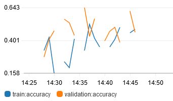
First thing out of the box is that the accuracy was low. Not only that, but the training accuracy was actually decreasing! This is bad because the training data have been seen by the algorithm previously during training and thus should have decent accuracy.
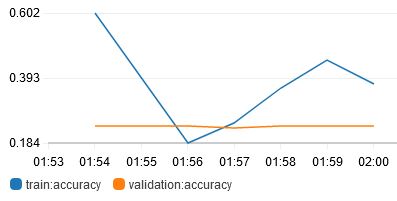
The decreasing and oscillating graph seems to indicate that the learning rate is too high, causing a divergence from the optimum, instead of a convergence. A more advanced optimizer such as Adam would also help, instead of just SGD.
I also noticed from the logs that the training accuracy increases within an epoch, but decreases sharply at the start of the next epoch, and this pattern continues.
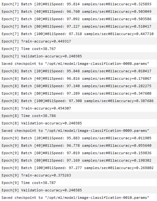
In this example, accuracy rises to 0.447 at the end of Epoch 7, but in Epoch 8, accuracy immediately drops to 0.01 and then rises again.
This seems to me like the algorithm is learning within an epoch, but immediately forgot or got confused at the start of the next epoch. I think this is caused by the ordered nature of the training data: in the lst file (v1), all daisy training data were provided first, then all the dandelion training data, then all the rose training data and so on. Shuffling of the data should help with this (and is always recommended anyway to remove any sort of unwanted ordering bias in the data).
Thus, I applied these changes:
- learning rate from 0.01 to 0.001
- optimizer from sgd to adam
- new lst file (v2) with the image order shuffled so that images from different classes are fed into the network randomly (rather than all of class 0 first, then all of class 1, then all of class 2 and so on)
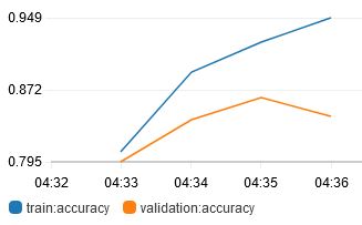
I was then able to start getting decent results, with increasing training accuracy.
Fine-Tuning: Learning Rate
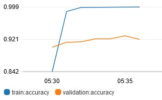
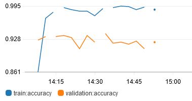
Now that I have good values to start tweaking, I started tuning specific hyperparameters. First of all, I tried different learning rates (lr):
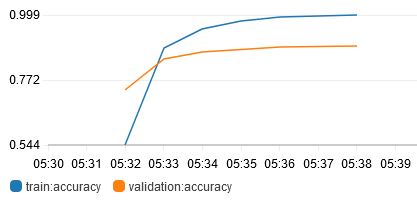
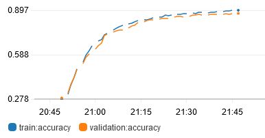
Also tried variable learning rates using lr_scheduler_factor and lr_scheduler_step. In the graph below, lr changed according to this:
- epochs 0 to 4: lr=0.0001
- epochs 5 to 9: lr=0.00001
- epochs 10 to 14: lr=0.000001
In the end, it appears that lr=0.0001 (constant) is the best learning rate to use.
Fine-Tuning: Num Layers
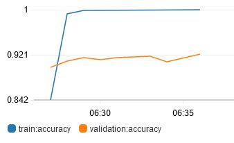
The next hyperparameter that I tried tuning was num_layers, which is basically the size of the ResNet. There are only a fixed number of sizes available to use: 18, 34, 50, 101, 152 and 200. Tried 50, 101 and 152.

From the results, larger networks do not necessarily correspond to better results. The best result obtained is from num_layers 50.
Fine-Tuning: Reverting Parameters For Confirmation
Just out of curiosity and for checking purposes, I turned off / reverted some parameters from the best model that I have so far, just to be sure that those settings are what I needed.
I tried changing the optimizer from Adam back to SGD:
It is much slower to train, and the accuracy is not as good as using Adam.
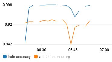
Also, I tried reverting my lst files back to v1, which is the file that had class-ordered training samples, and the results are bad as expected:
This concludes that shuffling of training data is necessary in the lst files.
Final model and hyperparameters:
The final trained model that I am using is v19
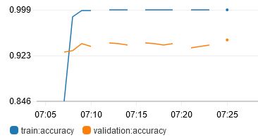
which uses these hyperparameters:
- epochs: 15
- learning rate: 0.0001
- mini_batch_size: 64
- num_classes: 5
- num_layers: 50
- num_training_samples: 3790
- optimizer: adam
- resize: 224
- use_pretrained_model: 1
Publishing The Model
Now that a good model has been trained, it’s time to deploy it. A SageMaker endpoint is first created, which basically allows for inference using the model within AWS. A serverless Lambda function is then created that queries the internal endpoint and returns a JSON object as the inference result. Lastly, AWS API Gateway is used to set up an external REST API that can trigger the Lambda function for an inference.
Now that there is an external REST API url, it is easy to send POST requests with image payloads (as base64 strings) via the usual avenues such as cURL, Postman or Python.
The request chain looks like this:
client → POST request → API Gateway → Lambda → Endpoint → model
after which the inference result will be passed back the chain in reverse from the model back to the client.
Testing The Model
I wrote a simple Python3 script to read in the test lst file that was created above, queried the REST API for each image to get a prediction, and then stored the actual-vs-prediction result in a confusion matrix.
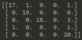
The accuracy for the 82 images in the test set is 0.922.
There are 7 images that are not predicted correctly:


A few observations about these cases that have failed predictions:
- Some of them are quite extreme edge cases
- The model is quite confident of many of these wrong predictions
- Tulip seems to be the wrong prediction for most cases
Conclusion
In this project, I have trained a flower image classification deep learning model using AWS SageMaker and associated ecosystem tools. Hyperparameter tuning was done to train a reasonably accurate model. Train, validation and test accuracies were 0.999, 0.949 and 0.922 respectively. A REST API was deployed for external consumption.